Top 10 Techniques to deal with Imbalanced Classes in Machine Learning!!

Yajendra Prajapati
Apr 15, 2023
8 min read

Class imbalance in machine learning refers to a situation where the classes in the training data are not represented equally. This means that one class may have significantly more samples than the other classes. This can be problematic because machine learning models trained on imbalanced data may have a bias towards the majority class, leading to poor performance on the minority class.

For example, suppose we are building a model to detect fraud in credit card transactions. Fraudulent transactions are rare, so the data may be highly imbalanced, with the majority of transactions being non-fraudulent. In this case, a model trained on this imbalanced data may have a high accuracy on non-fraudulent transactions but perform poorly on fraudulent transactions.

Techniques to handle Imbalanced Classes are: -

1. Random Under Sampling

Random under-sampling is a technique used to address class imbalance in machine learning. This technique involves randomly removing examples from the majority class until the dataset is more balanced between classes. The goal is to create a subset of the original dataset that has a similar number of examples for each class.

Here is an example to illustrate how random under-sampling works:

Suppose we have a dataset with 1000 observations, out of which 900 belong to class A (the majority class) and 100 belong to class B (the minority class). This dataset is highly imbalanced.

To balance the dataset, we can randomly select a subset of class A observations and remove them from the dataset. For example, we can randomly select 800 observations from class A and keep all 100 observations from class B. This will result in a new dataset with 900 observations, out of which 100 belong to each class. This new dataset is now more balanced, with an equal number of observations for each class.

2. Random Over Sampling

Random over-sampling is a technique used to address class imbalance in machine learning. This technique involves randomly replicating examples from the minority class until the dataset is more balanced between classes. The goal is to create a subset of the original dataset that has a similar number of examples for each class.

Here is an example to illustrate how random over-sampling works:

Suppose we have a dataset with 1000 observations, out of which 900 belong to class A (the majority class) and 100 belong to class B (the minority class). This dataset is highly imbalanced.

To balance the dataset, we can randomly select observations from class B and replicate them until we have a similar number of observations for each class. For example, we can randomly select 800 observations from class B and replicate them eight times each, resulting in 800 x 8 = 6400 new observations from class B. This will result in a new dataset with 7300 observations, out of which 3650 belong to each class. This new dataset is now more balanced, with an equal number of observations for each class.

Source - Research Gate

3. Random under-sampling with imblearn

Random under-sampling is a technique used to address class imbalance in machine learning, which involves randomly removing examples from the majority class until the dataset is more balanced between classes. In the imblearn library, this technique can be implemented using the Random Under Sampler class.

The Random Under Sampler class randomly removes samples from the majority class until it has the same number of samples as the minority class. The samples are removed randomly without replacement. This process results in a new dataset with an equal number of samples for each class.

Here's an example of how to use Random Over Sampler for random over-sampling:

from imblearn.over_sampling import RandomOverSampler

# assume X and y are the feature and target arrays, respectively
ros = RandomOverSampler(random_state=42)
X_resampled, y_resampled = ros.fit_resample(X, y)

4. Random over-sampling with imblearn

Random over-sampling is a technique used to address class imbalance in machine learning, which involves randomly replicating examples from the minority class until the dataset is more balanced between classes. In the imblearn library, this technique can be implemented using the Random Over Sampler class.

The Random Over Sampler class randomly replicates samples from the minority class until it has the same number of samples as the majority class. The new samples are created by randomly selecting samples from the minority class with replacement. This process results in a new dataset with an equal number of samples for each class.

Here's an example of how to use Random Over Sampler in imblearn:

from imblearn.over_sampling import RandomOverSampler

# assume X and y are the feature and target arrays, respectively
ros = RandomOverSampler(random_state=42)
X_resampled, y_resampled = ros.fit_resample(X, y)

5. Under-sampling: Tomek links

Under-sampling Tomek links is a technique used to address class imbalance in machine learning, which involves removing examples from the majority class that are close to examples from the minority class. This technique is based on the concept of Tomek links, which are pairs of examples from different classes that are closest to each other.

The basic idea of under-sampling Tomek links is to identify the Tomek links in the dataset and remove the majority class examples from the link. This process can help to reduce the overlap between the majority and minority classes, making it easier for the machine learning model to distinguish between them.

Here's an example of how to use Tomek Links in imblearn:

from imblearn.under_sampling import TomekLinks

# assume X and y are the feature and target arrays, respectively
tl = TomekLinks()
X_resampled, y_resampled = tl.fit_resample(X, y)

Source - MLWhiz

6. Synthetic Minority Oversampling Technique (SMOTE)

Synthetic Minority Oversampling Technique (SMOTE) is a popular technique used to address class imbalance in machine learning, which involves generating synthetic examples for the minority class. This technique creates new synthetic examples by interpolating between existing minority class examples. The SMOTE algorithm randomly selects an example from the minority class and then randomly selects one of its k-nearest neighbors. The synthetic example is then created by interpolating between the two examples.

The main idea behind SMOTE is to create new synthetic examples for the minority class that are similar to the existing examples, but not identical. This can help to reduce overfitting and improve the generalization performance of the machine learning model.

In imblearn, the SMOTE class can be used to implement the SMOTE algorithm. Here's an example of how to use SMOTE in imblearn:

from imblearn.over_sampling import SMOTE

# assume X and y are the feature and target arrays, respectively
smote = SMOTE(random_state=42)
X_resampled, y_resampled = smote.fit_resample(X, y)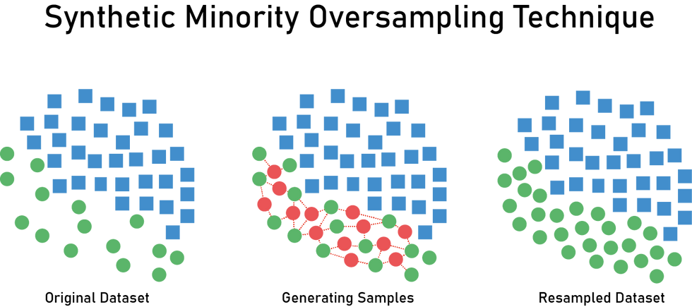

Source - Medium.com

7. NearMiss

Near Miss is a group of under-sampling techniques used to address class imbalance in machine learning. These techniques aim to reduce the size of the majority class by removing examples that are close to examples from the minority class. The basic idea is to keep only those examples from the majority class that are farthest from the minority class.

There are three variations of Near Miss under-sampling techniques:

NearMiss-1: In this technique, the majority class examples that are closest to the three nearest examples from the minority class are removed.
NearMiss-2: In this technique, the majority class examples that have the farthest average distance to the three nearest examples from the minority class are kept.
NearMiss-3: In this technique, the majority class examples that have the farthest average distance to the three farthest examples from the minority class are kept.

In imblearn, the NearMiss class can be used to implement these techniques. Here's an example of how to use NearMiss in imblearn:

from imblearn.under_sampling import NearMiss

# assume X and y are the feature and target arrays, respectively
nm = NearMiss(version=1)
X_resampled, y_resampled = nm.fit_resample(X, y)

8. Change the performance metric

When evaluating imbalanced datasets, accuracy is not always the most appropriate metric to use as it can be deceptive and may not reflect the true performance of the model, especially when the dataset has a significant class imbalance.

There are various other metrics that are more efficient than Accuracy.

Confusion Matrix: A table showing correct predictions and types of incorrect predictions.
Precision: It measures the percentage of true positives out of the total positive predictions. It is used when the focus is on minimizing false positives, such as in fraud detection or medical diagnosis.
Recall: It measures the percentage of true positives out of the total actual positives. It is used when the focus is on minimizing false negatives, such as in cancer diagnosis.
F1-score: It is the harmonic mean of precision and recall and is used when we want to balance the trade-off between precision and recall.
ROC AUC score: It measures the area under the receiver operating characteristic curve and is commonly used in binary classification problems.

9. Penalize Algorithms (Cost-Sensitive Training)

Penalizing algorithms or cost-sensitive training is a technique used to address the issue of imbalanced classes in machine learning. When the number of instances in one class significantly outweighs the number in the other class, standard machine learning algorithms may struggle to accurately classify the minority class.

Penalizing algorithms involve assigning a higher cost to misclassification of the minority class compared to the majority class. This higher cost serves as a penalty for misclassifying instances in the minority class, and can help the algorithm prioritize correctly classifying instances in the minority class.

For example, in a binary classification problem where the minority class is positive, the cost-sensitive approach involves assigning a higher cost to false negatives (instances that are actually positive but classified as negative) compared to false positives (instances that are actually negative but classified as positive). This way, the algorithm is encouraged to make more accurate predictions for the minority class.

10. Change the algorithm

Changing the algorithm can have a significant impact on imbalanced classes in a machine learning problem. Some algorithms may be better suited to handling imbalanced classes than others. For example, decision trees and ensemble methods such as random forests and gradient boosting are known to perform well on imbalanced datasets.

The choice of algorithm can also impact the extent to which penalizing techniques are necessary to address the imbalance. Some algorithms, such as support vector machines (SVMs), inherently take into account the distribution of classes in the dataset and may not require additional adjustment. In contrast, other algorithms like logistic regression or k-nearest neighbors (KNN) may require additional adjustments such as changing the decision threshold or using cost-sensitive techniques.

Pros and Cons of Under Sampling: -

Pros: -

Faster training: Down sampling the majority class reduces the number of training examples, which can lead to faster training times and lower computational requirements.
Reduced risk of overfitting: By reducing the number of majority class examples, undersampling can reduce the risk of overfitting on the majority class, which is often the case when the classes are imbalanced.
Better class separation: Downsampling the majority class can lead to better class separation and improved classification accuracy for the minority class.

Cons: -

Loss of information: Under sampling can lead to a loss of information in the majority class, which can lead to a reduction in overall model performance.
Increased risk of bias: Down sampling the majority class can result in a biased sample, which may not be representative of the original data distribution.
Increased variability: Under sampling can increase the variability of the model performance, as the random selection of examples from the majority class can lead to different results each time the model is trained.

Pros and Cons of Over Sampling: -

Pros: -

Improved performance: Oversampling can lead to improved classification accuracy for the minority class by increasing the number of minority class examples used for training.
Better representation: By increasing the number of minority class examples, oversampling can provide a better representation of the data distribution, which can lead to better model performance.
Reduced risk of bias: Oversampling can reduce the risk of bias in the training data, as it ensures that the model has sufficient examples of the minority class to learn from.